|

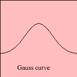
The Gauss curve is one of the most common distribution
function, especially in error theory, which lead to names like:
Mathematicians who worked on the curve were the English-French
mathematician de Moivre (in 1733), and later Laplace and Gauss.
For the distribution corresponding to the curve we find names as:
 The Gaussian distribution can be proved
(by the so-called Central Limit Theorem) in the situation that each
measurement is the result of a large amount of small, independent error sources.
These
errors have to be of the same magnitude, and as often positive as negative. The Gaussian distribution can be proved
(by the so-called Central Limit Theorem) in the situation that each
measurement is the result of a large amount of small, independent error sources.
These
errors have to be of the same magnitude, and as often positive as negative.
When measuring a physical variable one tries to eliminate systematic errors, so that only
accidental errors have to be taken into account. In that case the measured values will
spread around the average value, as a Gauss curve. It can be proved that in the case when
the average value of a measured value is the 'best value', a Gaussian distribution holds.
The 'best value' is here defined as that value, for which the chance on subsequent
measurements is maximal 1).
Because in general an estimation of errors is rather rough, the distribution to be used
has not to define the error very precise. More important is that the distribution is easy
to work with. And the Gaussian distribution has that quality in many situations.
Some real life examples of the Gauss distribution:
- distribution of the length of persons (given the sex)
- distribution of the weight of machine packed washing powder
- distribution of the diameter of machine made axes
Taking the definition of the standard deviation 2)
it can be seen that σ is the standard deviation in the Gauss
distribution of the form:

The points of inflection are situated at x = ± σ. For this
distribution about two of the three measurements has a distance less than σ from the maximum value. And about one of the twenty measurements
has a distance of more than 2σ.
Another interesting quality of the Gauss curve is that it is the only function which
remains unchanged for a Fourier transform.
Because its form the curve is also called the bell curve.
The curve can be signed to the flipped
Gauss curve.
notes
1) Squires 1972 p. 40.
2) The standard deviation of a distribution function f(x) is defined as:

|


 The Gaussian distribution can be proved
(by the so-called Central Limit Theorem) in the situation that each
measurement is the result of a large amount of small, independent error sources.
These
errors have to be of the same magnitude, and as often positive as negative.