
|
 |
 |
 |
 |
 |
 |
recurrent polynomial |
polynomial |
last updated: 2003-08-13 |
It's also possible to define a polynomial with a recurrent method, given a starting
function. There are an infinite number of polynomials y=f(x), where the nth is to derived
from former ones:
Fibonacci polynomial
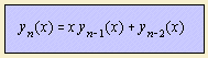 with y0(x)=0, y1(x)=1
Named to Fibonacci, famous of his Fibonacci series.
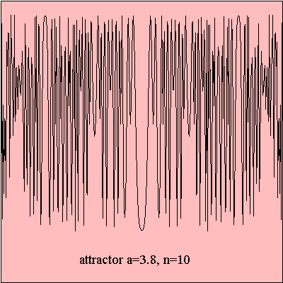
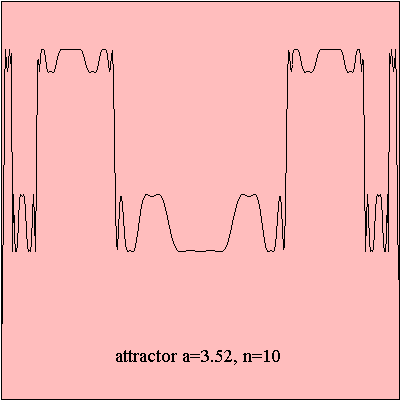
attractor
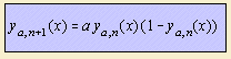 with ya,0(x)
= x
with ya,0(x)
= x
Above formula states the iteration of a parabolic function, giving a polynomial of degree
2n. For 0 < a < 4 convergence to one or more values may happen. Such
points of convergence 1) are called
attractors, later on this term was also given to the iterated curve.
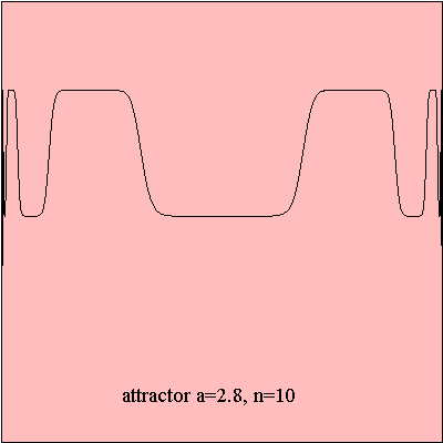
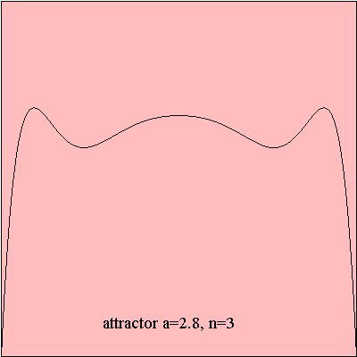 The character of these patterns depends strongly on
the value of the parameter a. For small values for parameter a, one sees just one point of
convergence. Enlarging parameter a, at a certain moment a doubling of attractors is to be
seen, the point of convergence seems to split, and later on again. Above some critical
value 2) no separate attractors are to be
distinguished, a chaotic region is entered.
The character of these patterns depends strongly on
the value of the parameter a. For small values for parameter a, one sees just one point of
convergence. Enlarging parameter a, at a certain moment a doubling of attractors is to be
seen, the point of convergence seems to split, and later on again. Above some critical
value 2) no separate attractors are to be
distinguished, a chaotic region is entered.
In fact we're looking at polynomials of a rather high degree 3), on a small part of the domain. It appears that
sometimes the generated polynomials have regions, where the function values are rather
constant. Sometimes the extremities are so close to each other, that it resembles to
chaos. This pattern changes with the parameter a.
The relationship can be used in population dynamics as a model (the Verhulst
model) to describe a retained growth, for insects or other creatures. The parameter a is a
measure of the fertility, for small values the species dies out. But there is also a
maximum population size, caused by the term 1 - f.
 The physicist Mitchell Feigenbaum discovered
that the quality of the maximum determines the behavior on the long term. It appeared that
parabolic behavior is not necessary parabolic, a quadratic maximum satisfies. Efforts are
undertaken to bridge the behavior of these curves to the chaos of the physical turbulence
(until now, without real success) 4).
The physicist Mitchell Feigenbaum discovered
that the quality of the maximum determines the behavior on the long term. It appeared that
parabolic behavior is not necessary parabolic, a quadratic maximum satisfies. Efforts are
undertaken to bridge the behavior of these curves to the chaos of the physical turbulence
(until now, without real success) 4).
These phenomena were quite popular in the beginning of the 20th century. From the 70s on
there is a revival, what produced a large stream of publications, especially in relation
to chaotic behavior. This renewed attention is partly understood by the easier access to
computing facilities, with whom the iterations can be easily calculated.
From these set of curves the fractal parabola bifurcation
can be derived.
notes
1) The attractor point will always lay on the line y=x.
2) of about 3.56.
3) the 10th iteration leads to a 1000th degree in x.
4) Hofstadter 1988 p. 395.